DASL Wiki

Author: Joao Matos Email: jcunha@id.uff.br
Date: Last modified on 6/8/2016
Keywords: Robotic Manipulator , Serial Arm, Denavit Hartenberg, Inverse kinematics

This page is to introduce the theory behind the robotic manipulators. It will be used the Denavit-Hartenberg parameters notation to describe the geometry of a serial chain of links and joints (Serial-Link).Using the robotic toolbox developed by Peter Corke (RVCtoolbox) we can visualize and understand more about the Denavit-Hartenberg parameters and how the process of the inverse kinematics works.

The understanding of this concepts are fundamental to understand the Image Based Servoing that will be implemented on the MM-UAV project.

More information about this concepts can be found at the book Robotics , Vision & Control ( Corke,2011).

Download the Toolbox here

Installation Instructions here

Dictionary with the functions syntax

Lego Robotic Manipulator

First we need to understand what a Serial Link Manipulator is.It can be described as a set of rigid bodies (LINKS) in a chain , connected by JOINTS. Each joint has one degree of freedom - which can be either Translational ( prismatic joint ) or Rotational ( revolute joint). Basically , moving each joint we change the position of the manipulator's end-effector (The tool at the end of the serial link manipulator designed to interact with the environment). Lets define that a manipulator has N joints numbered from 1 to N and N+1 links numbered from 0 to N. Also , the link number 0 will be the base ( fixed ) and the link number N will be the end effector. Each joint (j) will connect links (j-1) and j.

On the RVC toolbox we will see the serial link being described by a string containing “R”'s and “P”'s. This notation represent the type of each joint from the first to the last joint. For example , “RRRRR” represents a serial link with five revolute joints.

Denavit–Hartenberg notation:

Denavit–Hartenberg notation will set parameters to describe the links and joints of a serial link manipulator. The links parameters are two: its length (aj) and its twist (αj). The joints parameters are also two: its offset (dj) and its angle (θj). The joint type is characterized by (σ) , σ=0 is a revolute joint and σ=1 is a prismatic joint. For better understanding , lets take two consecutive joints (j) and (j+1). the end of the link (j-1) is attached to the joint (j) , the link (j) connect joints (j) and (j+1) - As said on before , each joint (j) will connects links (j-1) and (j) , each link (j) connects joints (j) and (j+1).Lets attach one coordinate frame to each of these joints (coordinate frame (xj-1 , yj-1, zj-1) and coordinate frame (xj,yj,zj)). SEE THE IMAGE BELLOW:

For this image the Denavit–Hartenberg parameters are:

• (aj): Is the displacement along the xj axis between the center of the frame (j-1) and frame (j).
• (αj): Is the Rotation around the xj axis that make the axis z(j-1) and z(j) to match each other.
• (dj): Is the displacement along the z(j-1) between the center of the frame (j-1) and frame (j).
• (θj): Joint angle rotation (around the z axis always - because we will always define the z axis as the axis of the joint rotation). This is the angle that we want to find when solving the Inverse Kinematic problem to find the desired pose of the robotic arm.
• (σ): Joint type: for revolute joints (rotational degree of freedom) σ=0 and for prismatic joints (translational degree of freedom) σ=1

Step by Step to find the DH notation for your robotic arm

It's very important that you follow some rules in order to guarantee that your DH notation is right. As the first step , we need to correctly define the frames on each joint , following some rules:

Four steps and rules to define the frame on each joint

1. You will define the z axes as the joints rotation axes (CCW). Start drawing only the z axis on all your joints, starting from z(0) at the base and going to z(….) at the end effector . DON'T FORGET that the z axis of the end effector must be in the same direction of the z axis of the last joint.
2. Now you will draw the x axes , the x axis must be perpendicular to both z(j-1) and z(j). Do it for every joint. If you have more than one direction that satisfy this condition , choose the direction that goes from z(j-1) to z(j) axes. DON'T FORGET that the x axis of the end effector must be in the same direction of the x axis from the last joint
3. Now you will draw the y axes.The y axis must follow the right hand rule , from z axis to x axis. And don't forget that the y axis of the end effector must be in the same direction of the y axis of the last joint.
4. Now that you drawn the three axis on every joint , you must check if the x(j) axis intersect the z(j-1) axis. To your DH notation be right , every x(j) axis must intersect the z(j-1) axis. If you don't have this , you must translate your (j) frame , in order to guarantee this intersection.

Steps and Rules to calculate the DH parameters after defining the frames

1. Start creating a table with the columns with the variables: | j | θ | α |d |a | and the rows with number from 1 to your last frame(end-effector). BE CAREFUL , we defined the frame on the base as j=0 , so you will not calculate DH parameters using directly the base frame !!! .
2. Calculate θ,α d, a following the definitions

• (aj): Is the displacement along the xj axis DIRECTION between the center of the frame (j-1) and frame (j).
• (αj): Is the Rotation around the xj axis that make the axis z(j-1) and z(j) to match each other.
• (dj): Is the displacement along the z(j-1) DIRECTION between the center of the frame (j-1) and frame (j).
• (θj): If you have only revolute joints , you can call them q1,q2,q3,q4…….

Now that you successfully defined each frame , you can calculate each DH parameter (θ, α ,d, a). The benefit of using the DH notation is that you can easily get the transformation from frames (j-1) and (j) inputting only this four parameter in a matrix. And after you have the matrices for every (j) , you can multiply all this matrices and get the transformation from the base to the end effector in only one matrix.

The transformation from link coordinate frame (j-1) to frame (j) can be defined in terms of elementary rotations and translations as shown bellow.

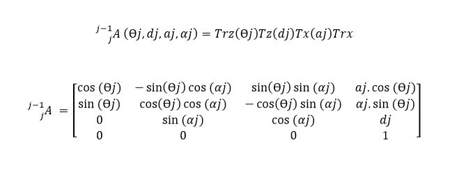
This can sound confusing but will be more clear on the next section examples. Also , this video is very didactic and helps you to understand what is the process to get the transform from the base to the end-effector in order to get the end-effector pose.

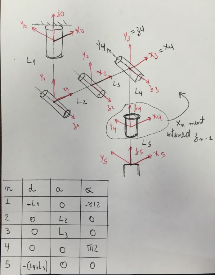
Following the step by step and rules presented previously, lets calculate the DH parameter for the serial arm available on the DASL at UNLV.

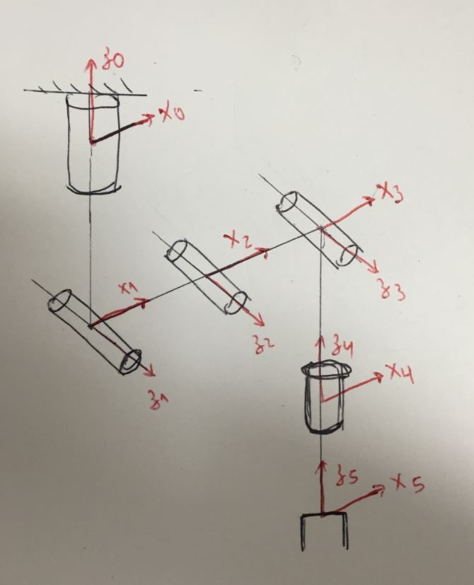
Defining the Frames

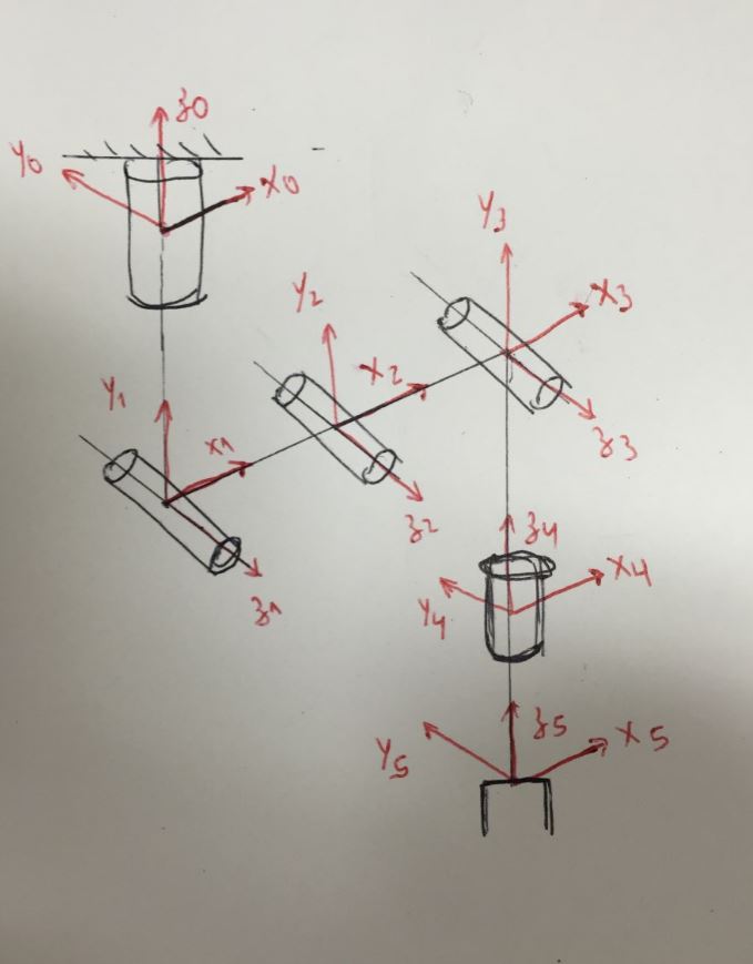
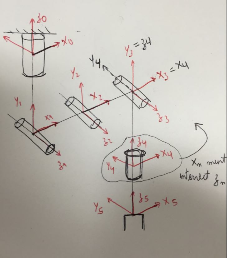
1→ drawing the z axes. 2→ drawing the x axes. 3→ drawing the y axes. 4→ checking if every x(n) axis intersect the z(n-1) axis. 5→ Change the axis that don't follow rule 4. 6→ Create the table and get the DH parameters.

We have many ways of defining the serial link on this toolbox. Lets see two easy methods:

Method 1 (creating a two links mechanism): Define each link using Denavit–Hartenberg and then create a serial link using these links. Open a new script on MATLAB and be sure that you included the folder with the RVC toolbox to the Matlab directory.

First lets define each link by its Denavit-Hartenberg parameters. It will be a two links mechanism,. <Code> %Defining each link %Link([THETA D A ALPHA SIGMA OFFSET(optional)]) ← Denavit- Hartenberg parameters

L(1) = Link([0 0 1 0]); L(2) = Link([0 0 1 0]); </Code>

Now we use the constructor SerialLink to create a serial link using the vector containing each link DH parameters .

<Code> %Creating using SerialLink Constructor %SerialLink(LINKS VECTOR , OPTIONS ).

method_1=SerialLink(L,'name','First Method'); </Code>

Run this code on a Matlab script and your serial link arm called first method example is done. You can type 'method_1' on the command window to check if the properties of your robot arm are correct.

As we can see the serial link called “First method” consist of two revolute joints (RR) and is defined following the standard Denavit-Hartenberg parameters (stdDH). (j) is the number of each link.

Observation: Instead of using the link angle as (θ) we often call each joint angle as (q). 'q' represents a generalized joint coordinate - which on the case of an all-revolute joints robot the joints coordinates are referred to as the joints angles. The values of each q will define the manipulator pose.

Method 2:(Our Legs motion) Define a starting coordinate frame at the base and describe each joint as a set of elementary rotations and translations (As shown in the first section)-we will do a transform for the whole system ( from the base to the end-effector). For example lets take the human leg. The hip can make the foot(end-effector) to go up and down , and go to left and right. The knee joint only make the foot go up and down. The foot can make the same movement as the hip joint (but lets omit the foot joint to simplify). Imagine this following image as a leg on the sitting position.

The coordinate frame is attached to the hip. L1 is the quadriceps length , joint 3 is the knee and L2 is the leg length. The foot would be joint 4 but is omitted here to simplify. As said before , the hip joint can make the foot to go up and down , forward and backward . Lets define two joints for the hip - First , joint 1 , will make the forward and backward movement ( q1 rotation about the z axis). The second hip joint will make the up and down movement (q2 rotation about the x axis). The knee joint only can make the foot to go up and down , so we have a q3 rotation about the x axis ) and this joint is not on the reference frame , so we will need to add a translation to this joint. * Remember all the rotations and translations are about a fixed reference frame.

Now lets define the set of rotation and translations transform that will represent the whole system. In order we will have:

• 1: Hip joint forward and backward → q1 rotation about the z axis - 'Rz(q1)'
• 2: Hip joint up and down → q2 rotation about the x axis - 'Rx(q2)'
• 3: The knee joint is translated by the quadriceps length in the y direction - 'Ty(L1)'
• 4: The knee joint up and down → q3 rotation about the x axis - 'Rx(q3)'
• 5: The foot joint is translated by the leg length in the z direction - 'Tz(L2)'

Open a new MATLAB Script and make sure that you added the RVC toolbox folder to the MATLAB path.

First we define the lengths and write the transform as a string, following the order (from the base to the end effector (from hip to foot )). <Code> L1= 0.5 %quadriceps length 0.5 meters L2= 0.5 %leg length 0.5 meters

%Write the set of rotation and translation transform transform='Rz(q1).Rx(q2).Ty(L1).Rx(q3).Tz(L2)'; </Code>

Now we can use a function from the toolbox to get the Denavit-Hartenberg factors from this transform. <Code> %Get the Denavit-Hartenberg factors dh_factors=DHFactor(transform); </Code>

We can get the necessary command to create a serial link using the following toolbox function: <Code> %Create the necessary command to create a serial link command=dh_factors.command('Second_Method'); </Code>

And finally we create our serial link evaluating the command that we created before. <Code> %Create the serial link called Second_Method Second_Method=eval(command); </Code>

As we can see , starting from a transform consisting of rotations and translations about a reference frame we got a serial link defined by DH parameters. In many cases is easier to follow this method , because is hard to see what is each DH parameters in an object with a lot of joints (will use a lot of frames and can be confusing).

Now that we have our serial link object ready , its time to plot it in a desired pose ( end effector position and orientation). Basically we have two methods : Forward Kinematics and Inverse Kinematics . Forward Kinematics is about use a set of joints angles and solve for the end-effector position. Inverse Kinematics is the inverse - using the end-effector desired coordinates , solve for the joints angles.

Foward Kinematics

In the Foward Kinematics problem we have the end-effector pose as function of joint coordinates. It can be computed for any serial link manipulator irrespective of the number of joints or the type of joints.

In practice , the pose of the end-effector (T) will be a product of the individual link transformations matrices ( see again the matrix on the “Denavit–Hartenberg notation” section).

Solving Foward Kinematics on MATLAB using RVC toolbox

As said , we want to know what will be the end-effector pose ( position and orientation ) given the generalized joints coordinate (q). Lets use the example from Method 1 of the previous section.

We start creating our Serial Link Manipulator ( it will be a two links mechanism called method_1).

<Code> L(1) = Link([0 0 1 0]); L(2) = Link([0 0 1 0]);

method_1=SerialLink(L,'name','First Method'); </Code>

We have two joints , that will result in two generalized joints coordinates (q1) and (q2). Lets assume q1=q2=0 , to know what will be the pose of the end effector we can use the solver '.fkine' to solve for the end effector pose. Also , we can use '.plot' after the serial link name to plot the end effector pose given the q1 and q2 angles. <Code> method_1.fkine([0 0])

method_1.plot([0 0]); </Code>

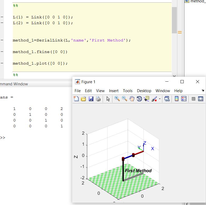
*The matrix outputted from the fkine solver is the homogenous transform that represents the pose of the second link coordinate frame of the robot (end-effector), T2.

Inverse Kinematics

The Inverse Kinematics problem is given the desired pose of the end-effector , what are the joints coordinates to make that pose? In general for some classes of manipulators no closed-form solution exists , necessitating a numerical solution.

Closed-Form Solution

A necessary condition for a closed-form solution of a 6-axis robot (most used in industry) is that the three wrist axes intersect at a single point (i.e the motion of the wrist joints only changes the end-effector orientation , not its translation). This kind of mechanism is known as spherical wrist.

In general ,for 6-axis robots , there are eight sets of joint coordinates that gives the same end-effector pose (because the inverse kinematics solution is not unique ). We usually call some particular solutions by names , such as right-handed or left-handed solutions (depending where is the arm in respect to the waist).

Solving Inverse Kinematics on MATLAB using RVC toolbox

Lets use as example a 6 joints robot ( Puma 560). The toolbox has the puma 560 model saved on its library , so we first start creating the puma 560 serial link . The command mdl_puma560 will load the puma 560 model and create a serial link object called p560 on the workspace. <Code> mdl_puma560 </Code>

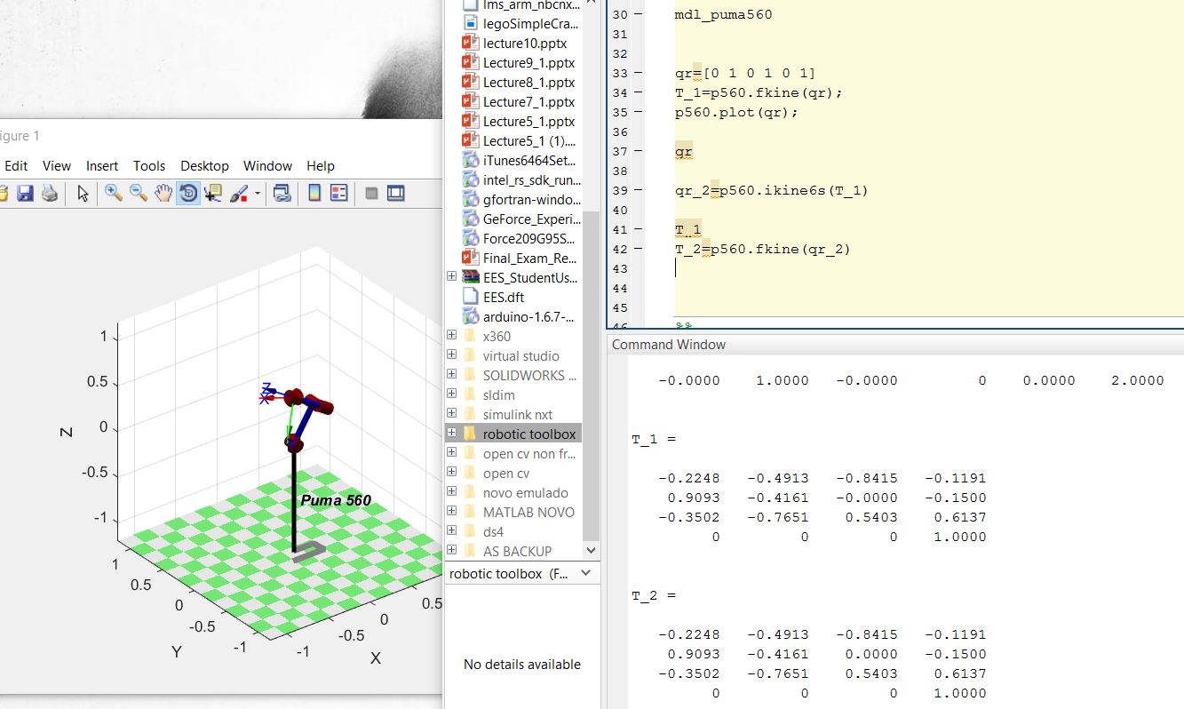
Now lets solve the Foward Kinematics problem and find the end-effector pose given qr=(0 1 0 1 0 1). <Code> qr=[0 1 0 1 0 1] T_1=p560.fkine(qr) p560.plot(qr); </Code>

And now lets solve the inverse problem , inputting the pose (T_1) and get the angles. For 6-axis robot there is a special solver called 'ikine6s' . For other number of joints you can use just 'ikine' , but you will need to define a submask vector , you can read more about it Here , on the ikine section. <Code> qr_2=p560.ikine6s(T_1) </Code>

You can check on the workspace that sometimes qr_2 will be different from qr depending on what angles you chose for qr. It's because the inverse kinematics problem on the closed-form has more than one unique solution (right-handed, left-handed , elbow-up , elbow-down , etc…). However , you can check that T_1 is equal to the solution T_2 obtained inputting the qr_2 angles.

<Code> T_2=p560.fkine(qr_2) </Code>

T_1 and T_2 must be the same end-effector pose. (same matrices).

If you followed the last topics on this page you already know how to create a serial Link based on its Denavit-Hartenberg parameters , so lets do this for the DASL serial arm. The code is:

<Code> %Creating the DASL serial arm on the RVC toolbox. %L(n)=LINK([theta D A alpha Sigma(optional) Offset(optional)])

L1=11; L2=15; L3=10; L4=21; L5=8; pi=3.1416;

q0=[0 0 0 0 0];

L(1)=Link([0 -L1 0 -pi/2 0]); L(2)=Link([0 0 L2 0 0]); L(3)=Link([0 0 L3 0 0]); L(4)=Link([0 0 0 pi/2 0]); L(5)=Link([0 -(L4+L5) 0 0 0]);

DaslArm=SerialLink(L,'name','DaslArm');

DaslArm.teach(q0)

</Code>

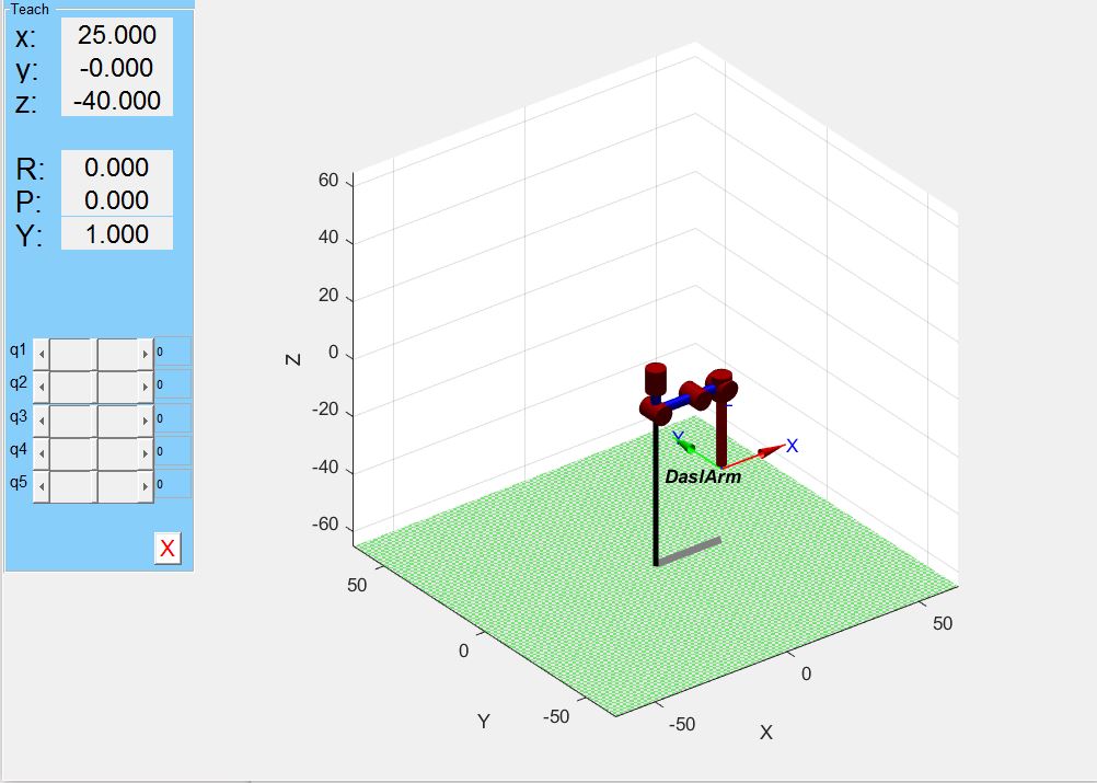
The teach command will create a window that allow you to change the q1,q2,q3,q4,q5 rotation and see how the arm moves , it's good to change this rotation by hand to check if your Denavit-Hartenberg parameters are OK.

If everything is moving as the arm moves , we can use the IK solver available on the RVC toolbox to get the joints angles given a desired end effector pose , you just need to add this code after defining your serial link object :

<Code>

%END EFFECTOR POSITION % trotx(angle) = rotate (angle) about the x axis % troty(angle) = rotate (angle) about the y axis % trotz(angle) = rotate (angle) about the z axis % transl(x,y,z) = pure translation of x , y , z % The end effector pose will be a combination of tranls and trot

%For example lets use a pure translation . T=transl(20,35,-30);

%IK SOLVER %Initial pose (all rotations = 0) q0=[0 0 0 0 0]; %Mask to be used on the IK solver (x y z rotx roty rotz) m=[1 1 1 0 0 0];

%Solving the IK and converting to degrees q_ikine=DaslArm.ikine(T,q0,m); q_degrees=q_ikine*(180/pi);

%Creating a trajectory from q0 to the IK solution %Time variable t=[0:0.05:4]; %trajectory q_TRAJ=jtraj(q0,q_ikine,t);

%Plot the result DaslArm.plot(q_TRAJ)

</Code>

This code will open a window to show the animation of the serial arm , going from an initial position q0 ( we defined as all the joint angles =0 ) to a final position - which is the IK solution. Is important to note that some end effector poses cannot be reached by the arm , so when you input these values , you will get some errors saying that the IK solver took more than 1000 iterations to find a solution and you will get an approximated solution. This IK solver available on the toolbox is not 100% accurate , the best choice is to program the IK solver by yourself , you can easily find a lot of algorithm to solve an IK problem on the internet.