DASL Wiki

This tutorial covers the use of harmonic functions to navigate a robot through an obstacle course. Harmonic potential fields overcomes many of the shortcomings of ordinary potential fields path planning algorithms, as it utilizes harmonic functions that rid of local minima within a plane.

—————————————————————————————————————————–

This tutorial's motivation is to first give an overview of properties of harmonic functions, and then demonstrate the ability of harmonic functions to alleviate some of the shortcomings typical potential fields path planning algorithms face. I will then explain and demonstrate the multi-panel approach for complex obstacle representation.

The rest of this tutorial is presented as follows:

• Harmonic Functions
• Properties of Harmonic Functions
• Uniform Flow
• Panel Method for Potential Fields
• Multi-Panel Method for Complex Obstacles
• Code
• Final Words

This work is presented in more detail in this paper .

—————————————————————————————————————————–

• Harmonic functions are multi-variable functions defined in terms of the laplacian.
• A laplacian is a special way to extend the second-derivative into multiple dimensions.
• Harmonic functions are functions where the laplacian is equal to zero (Δf = 0).

—————————————————————————————————————————–

• Mean-Value Property

• For a 2-dim potential function φ, the mean-value property states that value of harmonic function φ at a point (x,y) is equal to average value at φ over any circle around (x,y)

• Maximum Principle

• Maximum of a non-constant harmonic function occurs on the boundary

• Minimum Principle

• Minimum of a non-constant harmonic function occurs on the boundary

• These properties are useful for obstacle avoidance as harmonic function completely eliminates local minima, a major shortcoming of conventional potential field path planning algorithms.

• 
• The figure above and to the left represents an artificial potential field using harmonic functions, whereas the right represents that of an artificial potential field using non-harmonic function. There exists a local minima at (0,0) for the non-harmonic function but not so for the harmonic.
• You can also observe the minimum and maximum principles displayed in the figure. All maximum and minimums occur on the boundary of the potential field.

—————————————————————————————————————————–

• Harmonic Function useful for building artificial potential fields.
• In n=2 dimensions, if flow flows in directions which makes an angle α with x-axis, the potential function for uniform flow is:
• 
• U = magnitude (strength of uniform flow)
• With uniform flow, potential around a point is determined by strength of: uniform flow + strength of panel source.
• In the above equation φ,

—————————————————————————————————————————–

• The panel method is used to solve potential flow of a fluid around bodies of arbitrary shape.
• In this method, the surface of a body is covered by a finite number of small areas called panels.
• Each panel contains source or sink singularities which have a uniform density.
• In the picture below, a single panel is distributed with uniform sources with strength per unit length of λ.
• 
• The potential at any point (x,y) induced by the sources contained with a small element dl of the panel is:
• To find the induced potential function of the whole panel, take the integral over the length of the panel:
• Differentiation w.r.t. x and y gives the following expressions for the velocity components:

—————————————————————————————————————————–

• 
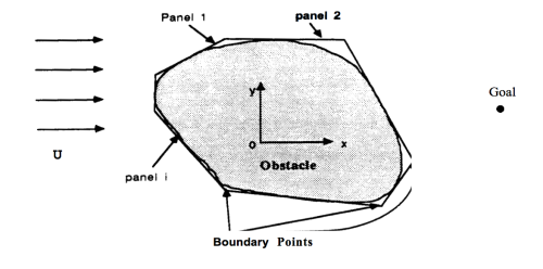
• Used to represent complex obstacles and cluttered environments.
• Obstacles approximated by set of panels numbered in clockwise direction.
• Each panel has own center point with a desired outward normal velocity as input variable.
• Boundary points are intersections of neighboring panels.
• If we let M = # of panels, and let λ₁, λ₂, … λ_M represent the source/sink strength per unit length of panel M, then the velocity potential at any point (x,y) by panel j is:
• where R_j is the euclidean distance between point (x,y) and the point (x_j, y_j) at panel j.

• We need an attractive potential at our goal point, where the potential has only one global minimum.
• This potential can be represented by a point singularity of sink, that acts like a drain in a sink, and has a strength of A > 0, and can be represented by:
• where R_g is the euclidean distance between point (x,y) and the goal point (x_g, y_g).

• The total potential due to obstacles, goal, and uniform flow is:

—————————————————————————————————————————–