This is an old revision of the document!
PID CONTROL
We can analyze the whole system into two distinct transfer functions , one for the ball and beam , and one for the motor. After , we can analyze the whole system putting these two transfer functions together in a block diagram.
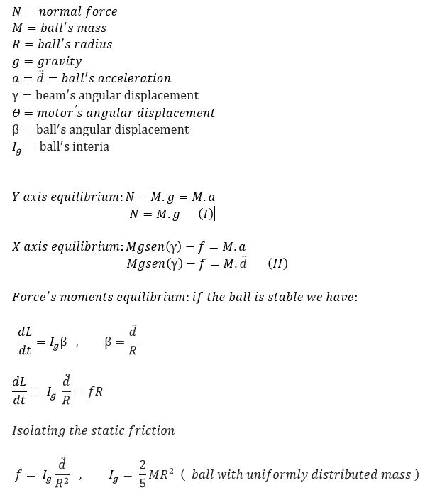
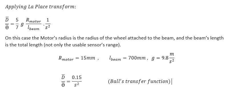
Ball and Beam Transfer Function Derivation
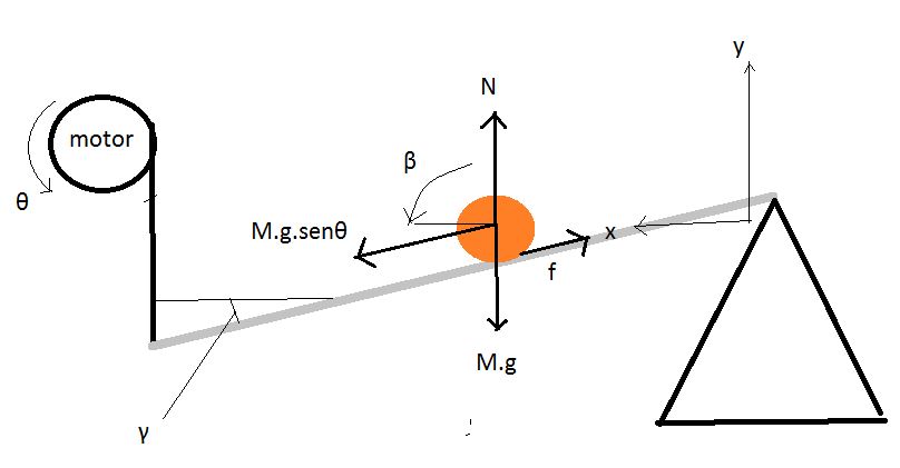
Analyzing the equilibrium we have:

Motor Transfer Function Derivation
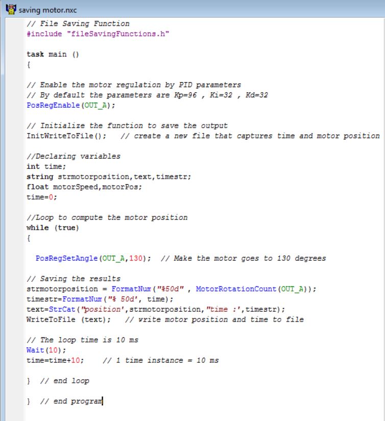
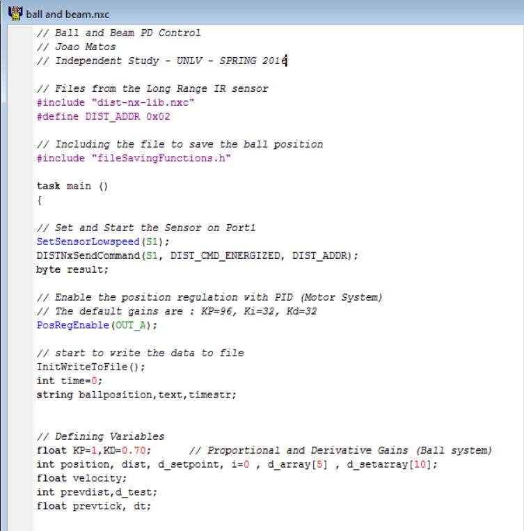
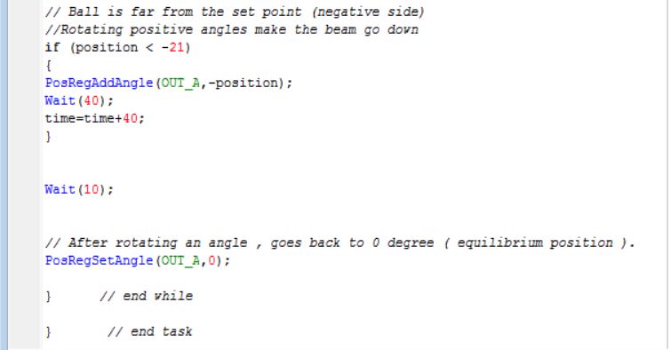
One easy way to get the motor's transfer function is to plot and analyze its response to an input , and by a graphical analysis get the parameters to derive its transfer function. We can program an algorithm to read and save ( using file saving functions ) the motor position during its operation. The following code was used to save and after plot the motor response until it get to the desired angle.The code makes the motor runs from 0 to 130 degrees, controlled by PID using the function “ PosRegEnable ” .
Plotting the results we have:
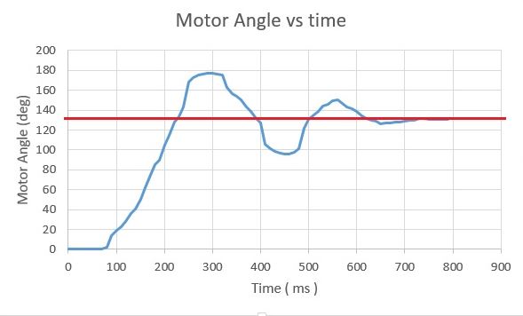
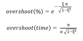
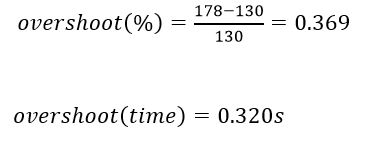
By the graphic response , we can assume the motor system as a second order system (because of the oscillatory and overshoot response). As known , a second order is characterized by two parameters , natural frequency (σ) and damping ratio (ξ).We can get these parameters by the following steps:
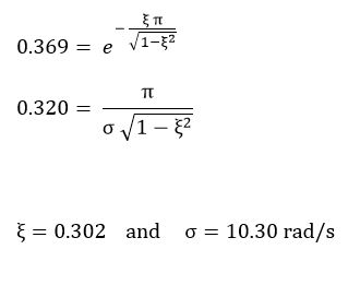
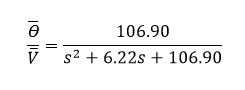
We know that a second order transfer function is:

So the motor's transfer function is:
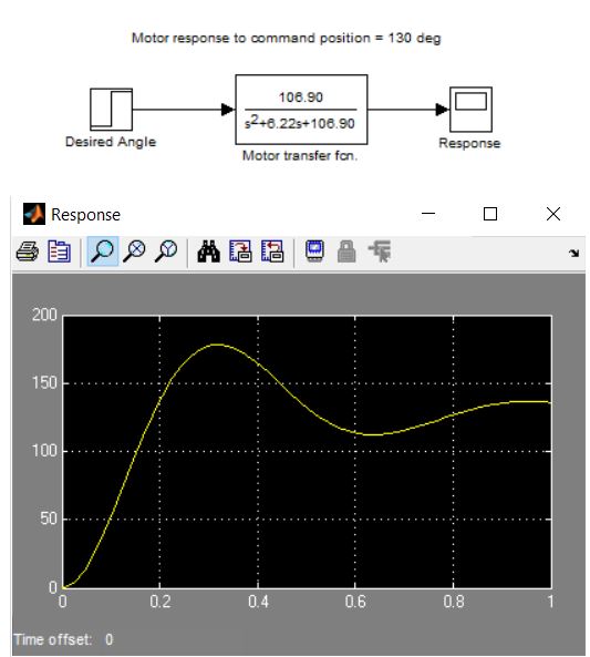
Motor system modeling on Simulink
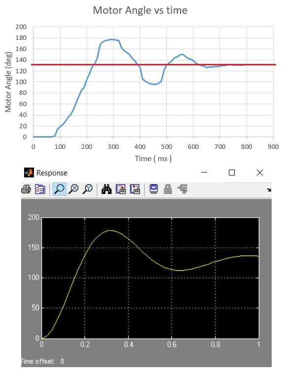
We can simulate the motor system on Simulink and compare the result to the experimental result , to verify if the derivation is correct.
Comparing both responses we can see that the derivation was correct.
SIMULATING THE WHOLE SYSTEM WITH PID CONTROL
We can simulate the whole system using the ball and beam together with the motor's transfer functions to simulate the real system. We can apply the PID control as well using Simulink. The block diagram and some results are shown bellow.
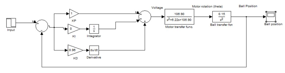
Simulation a disturbance on the system ( ball goes to 30 mm ) , we can see how the system will react in order to make the final ball position 0 mm.
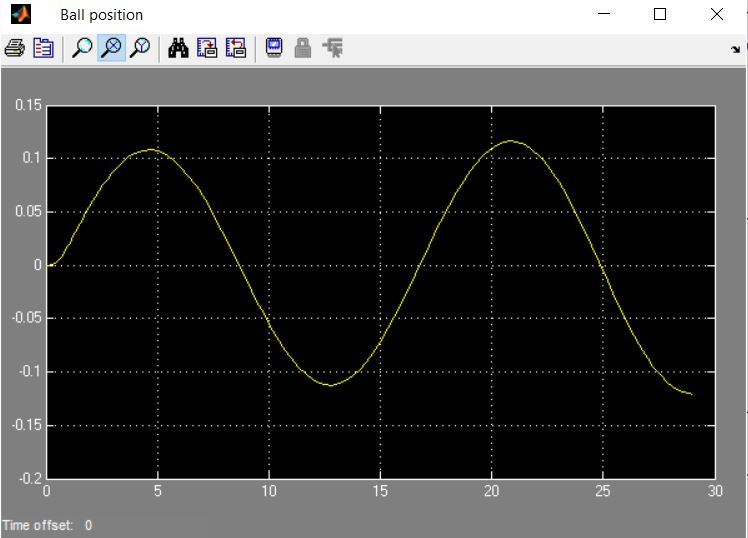
Using only proportional control ( system is unstable ).
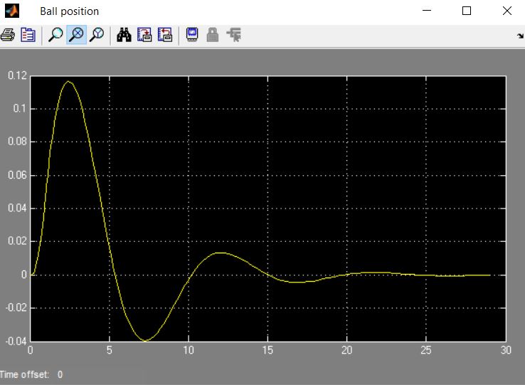
Using PD control (with non tuned gains (Kp=2,Kd=1). System disturbance rejection time: 4,6 seconds
Working Video / Simulating Disturbance
On the video ,was simulated first a heavy disturbance , and then two small disturbances.
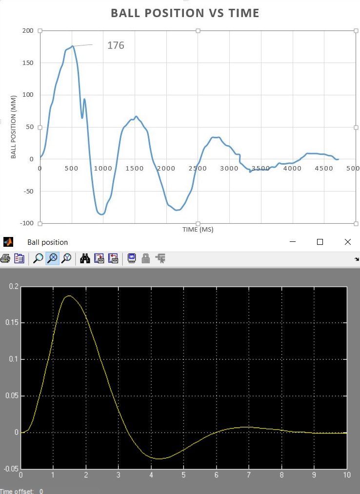
Comparison Simulink vs Real System
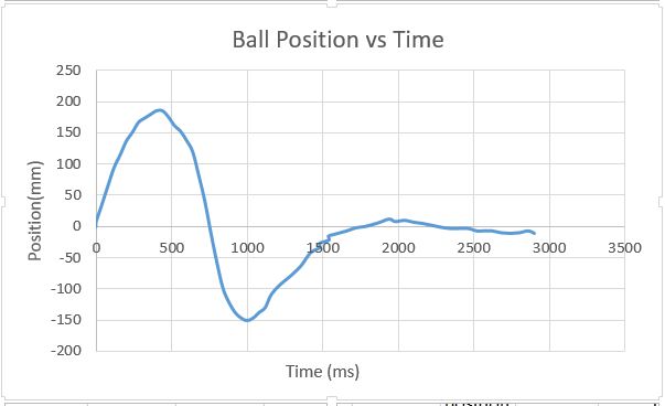
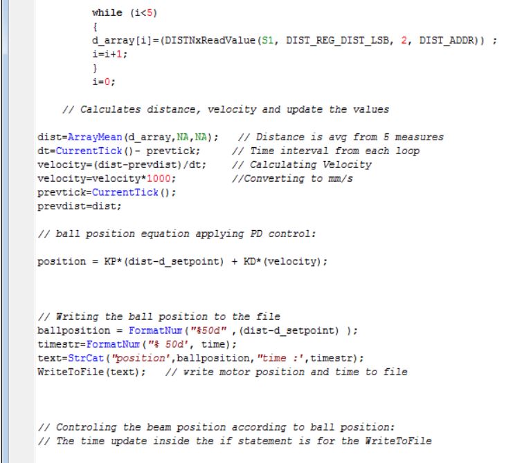
Introducing the a file saving function , the ball position over the time can be saved to a file and then plotted using an excel spreadsheet. Using KP= 1 and KI=0 and KD=0.76 and the disturbance shifting the ball to 176mm away from the setpoint.
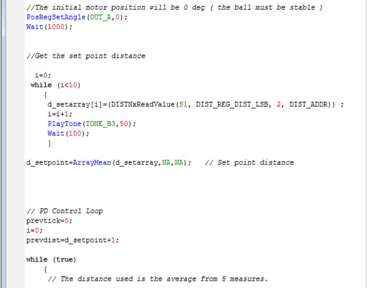
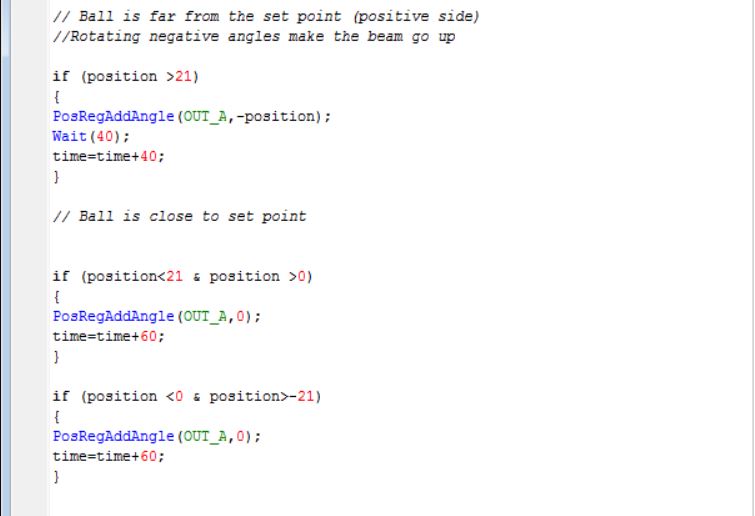
NXT CODE
TUNING THE CODE
After introducing the file saving function and the necessary commands to get the data , the system response was slowed down. ( oscillating more than before ). So i made some tuning:
- KP=1 and KD=0.60
- No waiting time inside the if statements
- 50ms waiting before starting the control loop again.
The new result is: