Author: Norberto Torres-Reyes Email: [email protected]
Date: Last modified on 09/06/18
Keywords: kinematics, planar, robotic arm, 2 link

The photo above depicts a diagram for a 2-link planar robotic arm. The big picture problem is to be able to obtain kinematic equations for any given degree of freedom robotic arm. This tutorial shows you how to obtain the kinematics of a 2-link robotic arm in order to solve for the joint angles given an arbitrary end-effector position.

This tutorial's motivation is to <fill in the blank>. Readers of this tutorial assumes the reader has the following background and interests:

* Knows How to Use Matlab
* Perhaps also knows linear algebra.
* Perhaps additional background needed may include knowledge of kinematics

The rest of this tutorial is presented as follows:

• Background And Theory
• Analytical Solution
• Numerical Solution
• Graphical Simulation
• Final Words

This section provides a short background of the problem and basic theory used.

Homogeneous Transformations



In this case, we will only consider 2-dimensional homogeneous transformations. First, we must introduce homogeneous coordinates:

Vector v = [x y w]^T , where scale factor w = 1

These coordinates are useful in applying rotations and translations and make transformations simpler than in Cartesian coordinates. We can apply an elementary rotation about the z-axis (normal to the page) with matrix:

[R_z] = [^Ax_B ^Ay_B ^Az_B]

Where ^Ax,y,z_B are the unit vectors along the x,y,z-axis of frame B w.r.t frame A. This results in:



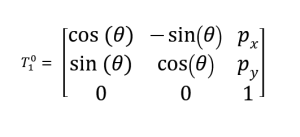
A translation vector p = p_xi + p_yj translates the origin of B from the origin of A. The given translation matrix P is given by:



Next, the translation matrix can be multiplied by the rotation matrix to obtain the complete homogeneous transformation matrix:



To obtain the coordinates for a given point p in frame B relative to frame A, the transformation matrix is multiplied by the vector of p in frame B. For example, in Matlab:

theta = 30*(pi/180);
Px = 2; Py = 3;
PframeB = [1; 4; 1];
T = [cos(theta) -sin(theta) Px; ...
     sin(theta)  cos(theta) Py; ...
     0 0 1];

PframeA = T*PframeB

PframeA = 
   0.8660
   6.9641
   1.0000

In the above example, frame B is translated in the (x,y) direction of frame A by (2,3) and rotated counter-clockwise by 30 degrees along the z-axis. The p vector in frame B has coordinates (1, 4) and the same vector in frame A has coordinates (0.8660, 6.9641).

To perform a combinations of rotations, translations, and/or transformations, the order of multiplication matters. For example, Rot_z(30)*Trans(2,3), means that frame B is rotated by 30 degrees about z-axis of frame A and then translated by (2,3) w.r.t frame B. On the other hand, Trans(2,3)*Rot_z[30] means frame B is translated by (2,3) w.r.t frame A, and then rotated by 30 degrees about z-axis of frame B.

If the transformation is about the new reference frame, then it is post-multiplied. If the transformation is about the old reference frame, then it is pre-multiplied.

For 3D rotations and translations, the following equations apply:



Forward Kinematics


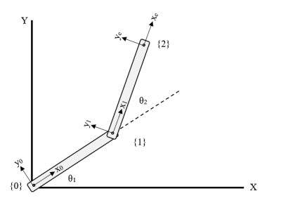
The image above shows a diagram of the 2-link robotic arm that will be used in this example.

The forward kinematics are used to calculate the joint angles. This is done using planar transformations to go from the origin plane to the end-effector plane. This can be done with arbitrary translations and rotations, but a more practical approach is to use the Denavit-Hartenberg parameters. Obtaining the parameters is discussed more below. First, we will focus on the specific translations and rotations.

Each relative transformation can be described by a matrix A:

^n-1A_n = Rot(z_n, theta_n)*Trans(0,0,d_n)*Trans(a_n,0,0)*Rot(x_n, alpha_n) , where n the number of links

Using Matlab, the relative transformation A can be calculated easily using symbolic variables (can also be done by hand):

>>syms theta d a alpha
>>Rotz = [cos(theta) -sin(theta) 0 0;...
          sin(theta)  cos(theta) 0 0;...
          0 0 1 0;...
          0 0 0 1];
>>Trans_d = [1 0 0 0;...
             0 1 0 0;...
             0 0 1 d;...
             0 0 0 1];
>>Trans_a = [1 0 0 a;...
             0 1 0 0;...
             0 0 1 0;...
             0 0 0 1];
>>Rotx = [1 0 0 0;...
          0 cos(alpha) -sin(alpha) 0;...
          0 sin(alpha) cos(alpha) 0;...
          0 0 0 1];
>> A = Rotz*Trans_d*Trans_a*Rotx
 
A =
 
[ cos(theta), -cos(alpha)*sin(theta),  sin(alpha)*sin(theta), a*cos(theta)]
[ sin(theta),  cos(alpha)*cos(theta), -sin(alpha)*cos(theta), a*sin(theta)]
[          0,             sin(alpha),             cos(alpha),            d]
[          0,                      0,                      0,            1]

Once each A matrix is obtained, the complete transformation T from frame {0} to frame {N} can be found through:

⁰T_n = ⁰A₁ * ¹A₂

Denavit-Hartenberg (DH) Parameters

The DH-parameters (theta_j, d_j, a_j, alpha_j) are obtained from a set of rules that can be easily referenced online. Also, this video is helpful in visualizing each parameter.
*The first parameter, the Joint Angle, is labeled on the diagram and is the angle from the previous x-axis to the new x-axis about the old z-axis.
*The Link Offset is the distance from the origin of the previous frame of reference to the new x-axis along the old z-axis.
*The link length is the distance between the old z-axis and the new z-axis along the new x-axis.
*Finally, the Link Twist is the angle from the old z-axis to the new z-axis about the new x-axis.

The parameters obtained can be substituted into the A that we calculated earlier for each transformation (with j = 1,2):

First, a triangle can be made from the two link arm with the above parameters specified.

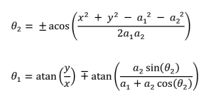
Recalling the cosine rule, A² = B² + C² - 2BCcos(a), the first equation can be found by:





From the above equation and diagram, we can gather that:



Finally, we have an analytical solution for each joint angle:

The following code uses the equations obtained in the analytical solution to calculate the joint angles for the 2-link mechanism.

clear; clc; format compact;

L1 = 2; %link 1 length
L2 = 3; %link 2 length
xPos = 2; %x position of end-effector
yPos = 1; %y position of end-effector

P = [xPos yPos]; %end-effector position vector

theta2 = acos((xPos^2 + yPos^2 - L1^2 - L2^2)/(2*L1*L2));
theta1 = atan2(yPos,xPos) - atan2((L2*sin(theta2)),(L1 + L2*cos(theta2)));

JointAngles = [theta1 theta2] %joint angle vector

In this case, the joint angles obtained for the first and second links are -1.1071 and 2.3005 radians respectively (or -63.4 and 131.8 degrees). The benefits of the analytical solution are rapid calculation times and precise answers.

As a sanity check, we can go back to the forward kinematics and apply the necessary transformations to calculate the position of the end-effector based on the joint angles obtained. For the above example:

>>Rotz1 = [cos(theta1) -sin(theta1) 0 0;...
          sin(theta1)  cos(theta1) 0 0;...
          0 0 1 0;...
          0 0 0 1];
>>Trans1 = [1 0 0 L1;...
           0 1 0 0;...
           0 0 1 0;...
           0 0 0 1];
>>Rotz2 = [cos(theta2) -sin(theta2) 0 0;...
          sin(theta2)  cos(theta2) 0 0;...
          0 0 1 0;...
          0 0 0 1];
>>Trans2 = [1 0 0 L2;...
           0 1 0 0;...
           0 0 1 0;...
           0 0 0 1];

>>T = Rotz1*Trans1*Rotz2*Trans2
T =
    0.3685   -0.9296         0    2.0000
    0.9296    0.3685         0    1.0000
         0         0    1.0000         0
         0         0         0    1.0000  

The final transformation vector shows that the coordinates of the end of the 2nd link are indeed (2,1), which is what we wanted.

We can also use the forward kinematics to plot a simple graph that shows the 2-link arm positions. With the following code the intermediate and final transformation matrices can be obtained.

>> T_01 = Rotz1*Trans1
T_01 =
    0.4472    0.8944         0    0.8944
   -0.8944    0.4472         0   -1.7889
         0         0    1.0000         0
         0         0         0    1.0000
>> T_02 = T_01*Rotz2*Trans2
T_02 =
    0.3685   -0.9296         0    2.0000
    0.9296    0.3685         0    1.0000
         0         0    1.0000         0
         0         0         0    1.0000
>> P = [0;0;0;1];
>> P1 = T_01*P; P2 = T_02*P;
>> plot([0 P1(1) P2(1)],[0 P1(2) P2(2)]); grid on;

The resulting plot will look like the following:

Matlab can be used to produce a graphical simulation of the 2-link arm mechanism for a given angle.

Hopefully, the information presented in this tutorial is enough for the reader to gain a good understanding of the background, theory, and practical knowledge required to apply this to a 2-link planar robot arm and possibly a 3-link planar arm.

For questions, clarifications, etc, Email: torresre@unlv.nevada.edu